
Loan Recovery System with Machine Learning
Introduction
Loan recovery is a critical challenge for financial institutions. Many traditional recovery methods, such as aggressive follow-ups and legal actions, often lead to customer dissatisfaction and increased costs. A Loan Recovery System with Machine Learning can optimize the process by predicting which borrowers are likely to repay and suggesting personalized recovery strategies.
In this end-to-end data science project, we will build an AI-powered loan recovery system using machine learning techniques. We will cover data preprocessing, exploratory data analysis (EDA), feature engineering, model building, evaluation, and deployment.

Why Build a Loan Recovery System with Machine Learning?
- Reduces Defaults: Predict borrowers who may default and take proactive actions.
- Optimizes Collection Efforts: Focuses recovery strategies on high-risk customers.
- Minimizes Legal Actions: Encourages amicable settlements instead of costly lawsuits.
- Enhances Customer Relationships: Provides personalized recovery plans rather than generic collection calls.
Step 1: Dataset Overview
The dataset contains crucial financial and borrower-related details:
| Column Name | Description |
|---|---|
| Borrower_ID | Unique ID for each borrower |
| Age | Age of the borrower |
| Gender | Gender of the borrower |
| Employment_Type | Type of employment (Salaried/Self-Employed) |
| Monthly_Income | Monthly earnings of the borrower |
| Num_Dependents | Number of dependents (family members financially dependent) |
| Loan_ID | Unique loan identifier |
| Loan_Amount | Total amount borrowed |
| Loan_Tenure | Loan period (months/years) |
| Interest_Rate | Interest rate on the loan |
| Loan_Type | Type of loan (Personal, Home, Auto, etc.) |
| Collateral_Value | Value of any collateral provided for secured loans |
| Outstanding_Loan_Amount | Remaining loan balance |
| Monthly_EMI | Fixed monthly installment for loan repayment |
| Payment_History | Past payment patterns |
| Num_Missed_Payments | Number of missed EMI payments |
| Days_Past_Due | Number of days loan payments are overdue |
| Recovery_Status | Target variable (1 = Loan Recovered, 0 = Defaulted) |
| Collection_Attempts | Number of times the bank attempted recovery |
| Collection_Method | Mode of recovery (Phone Call, Visit, Legal Notice) |
| Legal_Action_Taken | Whether legal action was taken (Yes/No) |
Step 2: Data Preprocessing
Load and Inspect Data
import pandas as pd

# Load dataset
df = pd.read_csv('loan_recovery_dataset.csv')

# Display basic info
print(df.info())
print(df.head())
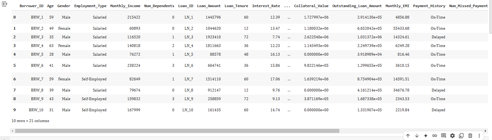
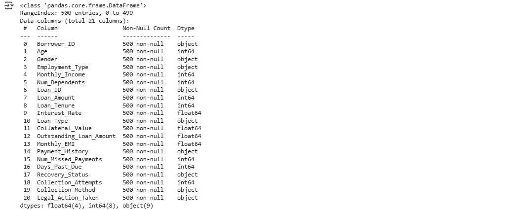
🔹 Why?
- Ensures the dataset is correctly loaded.
- Identifies missing values and data types.
Handling Missing Values
# Fill missing values for numerical columns with median
df.fillna({'Monthly_Income': df['Monthly_Income'].median(),
           'Collateral_Value': df['Collateral_Value'].median(),
           'Outstanding_Loan_Amount': df['Outstanding_Loan_Amount'].median(),
           'Num_Missed_Payments': 0,
           'Days_Past_Due': 0}, inplace=True)

# Fill categorical missing values with mode
df.fillna({'Employment_Type': df['Employment_Type'].mode()[0],
           'Collection_Method': df['Collection_Method'].mode()[0]}, inplace=True)

# Convert categorical variables to numerical
df['Employment_Type'] = df['Employment_Type'].map({'Salaried': 1, 'Self-Employed': 0})
df['Gender'] = df['Gender'].map({'Male': 1, 'Female': 0})
🔹 Why?
- Missing numerical values are replaced with median to prevent data skew.
- Categorical values are converted into numerical formats.
Step 3: Exploratory Data Analysis (EDA)
Visualizing Loan Recovery Trends
import matplotlib.pyplot as plt
import seaborn as sns

# Loan Recovery Distribution
sns.countplot(x='Recovery_Status', data=df, palette='coolwarm')
plt.title('Loan Recovery Status')
plt.show()
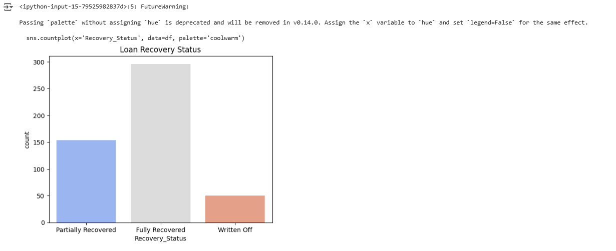
🔹 Insight:
- A highly imbalanced dataset may require SMOTE (Synthetic Minority Over-sampling Technique) for better model training.
Feature Correlation Heatmap
plt.figure(figsize=(12, 6))
sns.heatmap(df.corr(), annot=True, cmap='coolwarm')
plt.title('Feature Correlation')
plt.show()
# Select only numerical features for correlation analysis
numerical_features = df.select_dtypes(include=np.number).columns
correlation_matrix = df[numerical_features].corr()

plt.figure(figsize=(12, 6))
sns.heatmap(correlation_matrix, annot=True, cmap='coolwarm')
plt.title('Feature Correlation')
plt.show()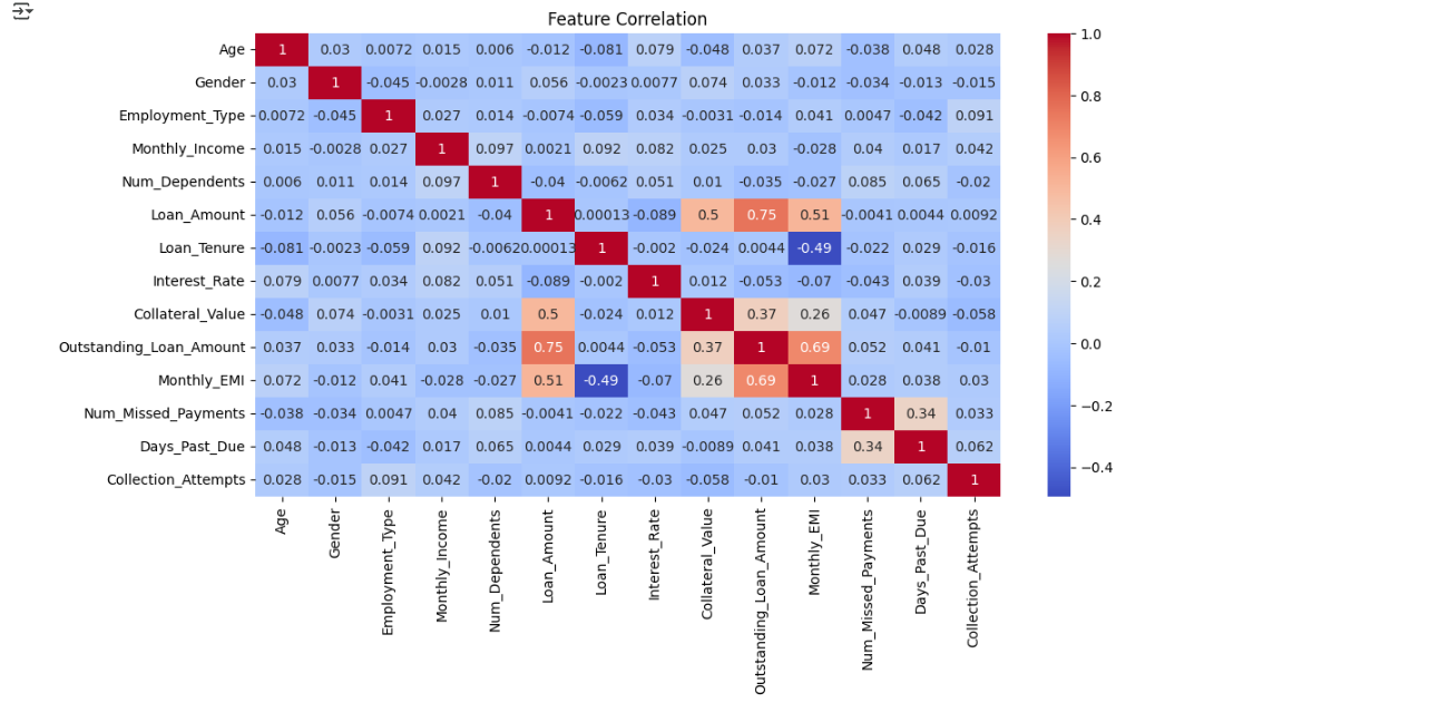
🔹 Insight:
- Features like Num_Missed_Payments and Days_Past_Due have a high correlation with loan recovery.
Step 4: Feature Engineering
Create New Features
# Debt-to-Income Ratio
df['Debt_to_Income'] = df['Outstanding_Loan_Amount'] / df['Monthly_Income']

# Loan Risk Score (Custom Formula)
df['Loan_Risk_Score'] = df['Interest_Rate'] * df['Num_Missed_Payments'] / df['Loan_Amount']
🔹 Why?
- Debt-to-Income Ratio helps assess repayment capacity.
- Loan Risk Score quantifies loan risk based on past defaults.
Step 5: Model Training
from sklearn.model_selection import train_test_split
from sklearn.ensemble import RandomForestClassifier
from sklearn.metrics import accuracy_score, classification_report
from sklearn.preprocessing import LabelEncoder # Import LabelEncoder

# Define features (X) and target (y)
X = df.drop(['Borrower_ID','Legal_Action_Taken' , 'Loan_ID', 'Recovery_Status'], axis=1)
y = df['Recovery_Status']

# Convert 'Payment_History' to numerical using Label Encoding before one-hot encoding
le = LabelEncoder() # Create a LabelEncoder object
X['Payment_History'] = le.fit_transform(X['Payment_History']) # Fit and transform the column

# Convert categorical features to numerical using one-hot encoding
categorical_features = ['Loan_Type', 'Collection_Method', 'Payment_History']
X = pd.get_dummies(X, columns=categorical_features, drop_first=True)

# Split into training and testing sets
X_train, X_test, y_train, y_test = train_test_split(X, y, test_size=0.2, random_state=42)

# Train RandomForest Model
model = RandomForestClassifier(n_estimators=100, random_state=42)
model.fit(X_train, y_train)

# Make predictions
y_pred = model.predict(X_test)

# Evaluate Model
print("Accuracy:", accuracy_score(y_test, y_pred))
print(classification_report(y_test, y_pred))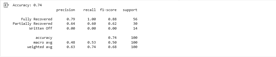
🔹 Why Random Forest?
- Handles both categorical and numerical features efficiently.
Step 6: Model Deployment
import joblib

# Save the trained model
joblib.dump(model, 'loan_recovery_model.pkl')
print("Model saved successfully!")
🔹 Why?
- Enables integration into loan management systems or web applications.
Real-World Applications of Loan Recovery System with Machine Learning
1️⃣ Banking & NBFCs: Predict loan recovery and optimize collections.
2️⃣ Microfinance Institutions: Provide customized repayment plans.
3️⃣ E-Commerce & Fintech: Automate risk assessments for BNPL (Buy Now, Pay Later) schemes.
Conclusion
A Loan Recovery System with Machine Learning enhances loan repayment predictions, reduces defaults, and improves customer experience. By implementing data-driven recovery strategies, banks and financial institutions can optimize debt collection while maintaining customer trust.
💡 Next Steps? Try experimenting with deep learning models or NLP for sentiment analysis of borrower responses to further enhance the system. 🚀


